Earned autonomy: a deployment doctrine for AI in the physical world

Before AI takes the next order

Consider an illustrative^† Friday afternoon. A dispatcher is arranging a two-person appliance delivery to a building that stops accepting deliveries at 4 p.m. Provider A quotes $84 and Provider B quotes $87; both show a delivery window ending before the cutoff. The dispatcher chooses B because A has just called to say its earlier job is running late. The AI recommends A because that update never reached the system. On screen, it looks like a three-dollar saving. To the dispatcher, it looks like a risk to the customer's promise.

The dispatcher's choice costs three dollars more, but it accounts for a delay the system has not seen. Judging the AI only on price would miss that distinction. Judging it only on whether it matched the dispatcher would tell us little about why the choices differed. Before the AI executes orders on its own, the team needs to understand differences like this one and know whether its recommendations hold up under real operating conditions.

We call this approach earned autonomy: authority is granted for a defined segment of an operation, against evidence thresholds agreed before evaluation, with automatic withdrawal when a hard rule is breached. The system first decides alongside dispatchers, then executes approved decisions under Review, and finally earns authority within the segment's rules. Agreement helps open the first gate; actual outcomes must open the last. Every decision leaves a record of the alternatives, constraints, and reasons that shaped it.

1. The deployment gap

Machine learning has a well-documented gap between benchmark performance and production readiness. Breck and colleagues at Google described teams scoring models on held-out data and then discovering that testing the model was the smallest part of testing the system.^[1] The appliance order makes that gap concrete: the model can compare every quote correctly and still miss the phone update that changes the call.

A dispatch decision commits real dollars to a provider, attaches a delivery promise to a real customer, and closes off alternatives that were not chosen. A wrong sentence can be regenerated. A wrong dispatch is a refund, a missed window, and a customer who remembers.

When a system is sold with full authority on day one, with instructions to set the objective, connect the account, and trust the machine, the operation is asked to rely on whatever the vendor's benchmark claimed. We call this pattern granted autonomy, and it has the order of operations backward. Authority should be the output of a measurement process, not the default state of an integration.

2. What older fields already know

Fields that put automation in front of physical risk offer three structural lessons that translate well to dispatch.

Authority is staged, never binary. Aviation evaluates automation within defined operating envelopes, and autonomous-driving safety evaluations examine performance within defined operating domains.^[2][3] The dispatch lesson is straightforward: authority for routine local orders does not establish readiness for an appliance installation with a two-person crew and a hard building cutoff. Wider permission requires evidence for the wider scope.

Evidence is comparative and gathered in the production distribution. Medicine formalized one version as the non-inferiority trial: a new treatment is asked to meet a justified, pre-specified margin against the standard of care.^[4] Production ML uses shadow deployment to run a candidate beside the incumbent on live traffic, without giving the candidate authority.^[1] Experimentation practice adds the discipline of setting decision criteria before the results arrive, because post-hoc thresholds are how organizations fool themselves.^[5] For the installation segment, that means agreeing on acceptable performance before inspecting the AI's calls.

Reversal is engineered, not negotiated. Circuit breakers, automation disconnects, and software rollbacks offer a common operating lesson: build the withdrawal path before expanding authority. If an autonomous installation breaches a hard dock cutoff, the team should already know what stops, where the next orders go, and who takes over.

Earned autonomy is not an invention. It brings these commitments into commerce operations. What's curious is how rarely it reaches commerce: the industry that would never let an uncertified autopilot fly a plane routinely lets an unevaluated model dispatch its orders.

3. The doctrine, stated

Earned autonomy is five commitments:

The three operating stages make these commitments tangible. In Shadow, the dispatcher books B while the system's choice of A is recorded. In Review, the system proposes A and the dispatcher overrides it, recording the delay call. In Autonomous, the system executes within the approved segment and rules, with monitoring and intervention in place.

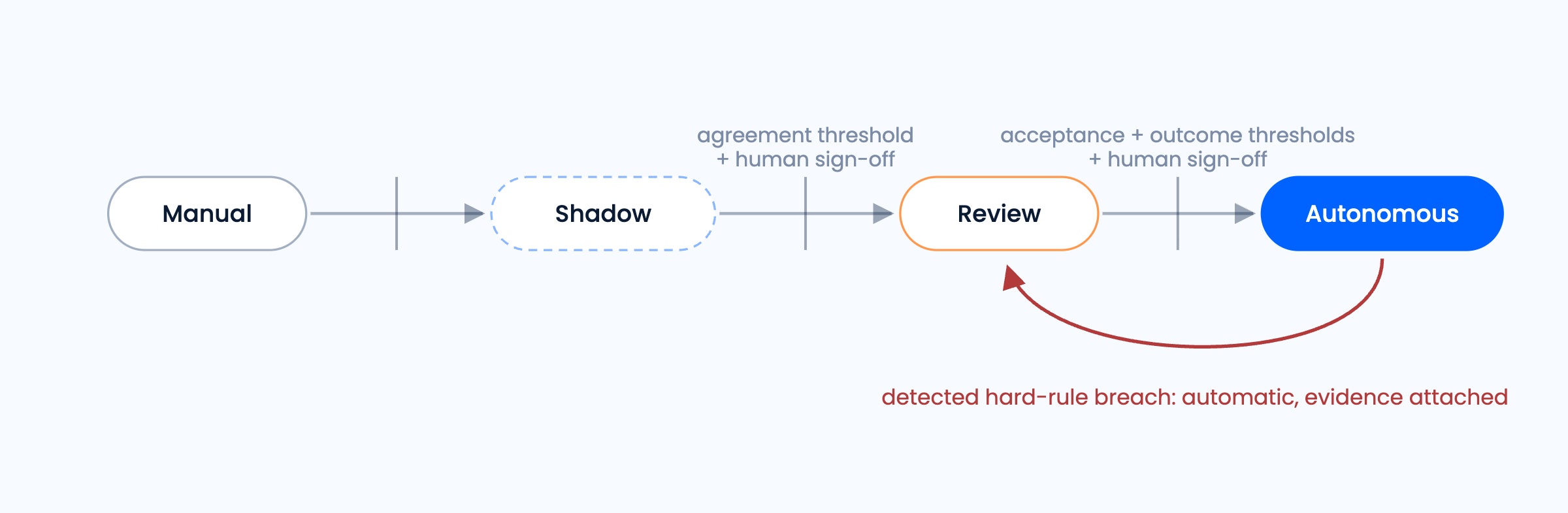
The appliance segment cannot make that last step while material updates routinely fail to reach the system. Updates like A's phone call must reliably arrive, or the system must identify affected orders and return them to a dispatcher, with the fallback demonstrated in practice. More authority follows evidence that the gap is controlled, rather than merely a higher match rate on easier orders.

The remainder of this note examines the parts that require statistical care: what counts as agreement, how much evidence is enough and in what units, what the system's own outcomes must show before full authority, why promotion and demotion are asymmetric, and why the evidence must be live.

4. The unit of trust: segments

Aggregate metrics are where deployment failures hide. Suppose an operation records 1,000 paired decisions: 900 local deliveries and 100 scheduled installations. The AI agrees with dispatchers on 798 local deliveries and 52 installations:

The overall number is dominated by the frequent work. It conceals a segment where almost half the calls differ and where the reasons need examination before granting authority. Disagreement does not itself prove the system is wrong, but the pooled average does not answer the installation question. Pooled results can obscure differences between subpopulations, a concern related to the broader hazards of aggregation.^[6]

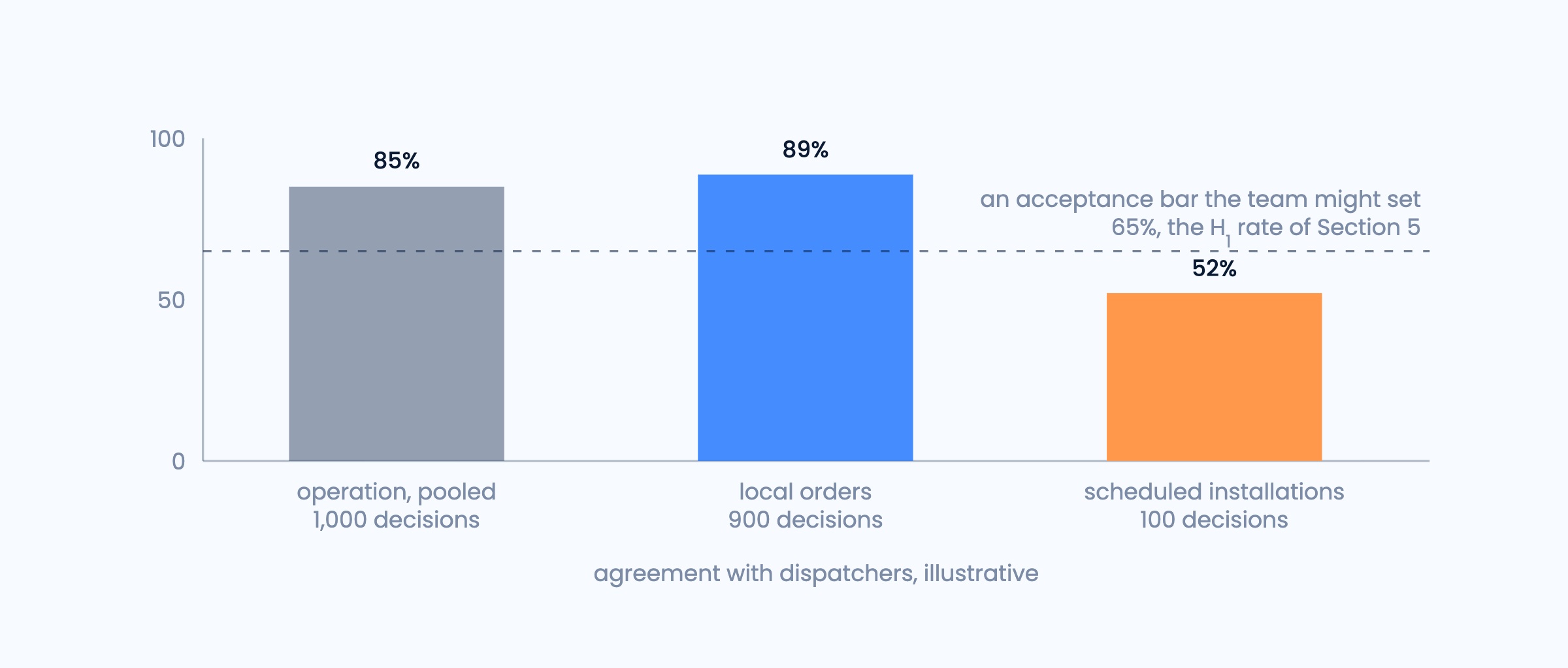
The doctrine makes the evidentiary unit and the authority unit the same object. A segment is defined by similar operating behavior: local orders under ten miles from one store, two-person deliveries within a defined service area, or parcel orders with two-day promises. Geography, order requirements, providers, and service commitments may all matter to the boundaries; a category name alone does not establish that its orders behave alike.

Each segment carries its own record, thresholds, and mode. Authority granted to one segment says nothing about another. Authority is never inherited. When a material constraint change redraws the segment map, the new segment's evidence clock starts at zero, however trusted its neighbors. The earlier record remains useful context, but it does not carry authority into the changed operation, because performance under the earlier distribution does not establish readiness under the new one.^[7]

5. Measuring agreement

In Shadow, the system's call is written beside the dispatcher's on live orders. The natural statistic is the match rate, but “match” needs a definition that respects how dispatch works: two decisions can differ in provider while being operationally comparable.

Define the decision and the match

Let a dispatch decision be the tuple:

Record exact-provider agreement separately from decision-equivalent agreement. Two different-provider calls qualify as decision-equivalent only when both are feasible under the segment's policy and their cost and promised-window differences fall within agreed tolerances:

Here, ε_c is the allowed cost difference, and ε_t is the time tolerance; both are set per segment alongside the promotion criteria. Feasibility and hard-rule compliance need independent checks even when the provider matches exactly.

Because a band can decide a promotion, the record reports both agreement measures and shows sensitivity to the bands. Cost and window deltas remain visible on equivalence matches as well as divergences: a $3 gap inside a band is still a $3 gap in the ledger. A promotion that would not survive a reasonable change in bands should be shown to the team as such.

Compare the options that were actually available

An order enters the agreement denominator only when both sides produce a call under the same constraint version, with timestamps and the option set each saw. Orders one side never saw prove nothing about agreement. A divergence is graded only if the system's alternative was still available when the dispatcher decided; a quote that expired between the two calls is not a saving anyone could have taken.

On the appliance order, the dispatcher flags the delay call as information outside the system's record. That pair is excluded from the agreement statistic but retained in the ledger, with the reason. Before evaluation, the team sets a maximum exclusion rate for the segment; exceeding it blocks promotion. Otherwise, the system could appear ready by passing on the orders where it had complete information while repeatedly missing the consequential ones.

Divergences are not merely counted. Each is recorded with its signed cost delta, the change in promise risk, and the reason for the difference.

Measure productive disagreement

Consider a second appliance order with no delay call, where both providers meet the requirements and independent operating evidence supports comparable service. Choosing A may then represent a genuine three-dollar opportunity, rather than an information gap.

A divergence is productive if an independent assessment, using what was knowable at decision time and realized outcomes where the record permits, favors the system's call. The productive-disagreement rate is:

This addresses the objection that matching the incumbent merely caps the system at the incumbent. Agreement is how a system earns authority; productive disagreement is why granting it was worth anything. Both compare the system with people; whether it improves the operation is a question about outcomes, which Section 6 makes a gate of its own. Ungraded disagreements remain visible so the team can see the limits of the comparison.

Correct for agreement expected by chance

Raw agreement flatters small choice sets. If a segment has two viable providers and dispatchers choose one most of the time, a system repeatedly choosing that provider can agree often without demonstrating much order-specific judgment. That concentration may be entirely sensible for the work; the question is what the match rate establishes.

Cohen's kappa discounts agreement expected from the two decision-makers' marginal provider-choice frequencies:^[8]

Here, p_o is observed agreement, while p_e is expected agreement under independent choices with those same frequencies. For example, if dispatchers choose B on 75% of orders and the system chooses B on 60%, with only A and B available:

With observed agreement p_o = 0.72:

Raw agreement remains 72%; kappa is another diagnostic, not a replacement agreement percentage or a measure of economic value. It shows how much agreement exceeds the baseline implied by those choice frequencies.

The promotion test can run on raw agreement under an appropriate statistical model, while κ is reported beside it per segment. The team may set a κ floor so that agreement explainable by one dominant provider cannot promote a segment on its own. With a floor of 0.40, this segment's 0.378 would block promotion even at 72% raw agreement. Kappa's limitations under imbalanced choices remain an open issue in Section 12.

Count evidence in decisions, not calendar time

The installation team now has a practical question: how many paired calls would make its agreement rate precise enough to judge?

Denominate in decisions, not calendar time, because observations build the evidence. Under an independent binary-observation model, the approximate standard error of an estimated agreement proportion is:

At an illustrative p̂ = 0.60 over n = 150 decisions:

Whether that precision suffices is a risk decision. Thresholds belong to the merchant, per segment; the examples in this note are not product constants.

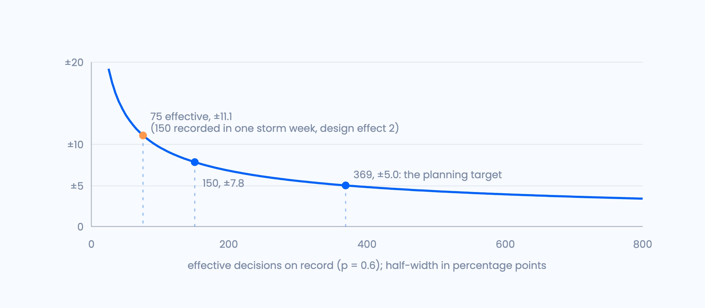
Run the formula backward to plan. Under the same independent model, pinning agreement within ±E = 5 points needs

Discount evidence that arrives in clusters

Decisions are the currency, but they are not independent coins. Suppose half those installation orders arrived during one storm week, when the same provider repeatedly lost capacity. The raw count is still 150, but many decisions share the same shock. They carry less independent information than the count suggests.

The doctrine therefore adds a minimum number of distinct operating days and accounts for clustering when estimating uncertainty. Effective sample size, written n_eff, expresses how much information a dependent sample carries relative to independent observations. One useful explanatory relationship is:

If an illustrative design effect were 2, then 150 recorded decisions would provide roughly the information of 75 independent ones:

That corresponds to an approximate interval of 60% ± 11.1 percentage points, wider than the independent calculation. Planning runs the same way in reverse: at a design effect of 2, the ±5-point target above takes roughly 369 × 2 ≈ 740 recorded decisions. The design effect must be estimated or justified; two is an example, not an automatic storm adjustment. Clustering can span several days, so grouping by day alone may not capture all dependence. A smaller effective count explains the issue but does not, by itself, validate a sequential test.

The operational implication is clear: a low-volume segment takes longer to earn the same certainty, and a busy but unusual week earns less certainty than its raw count suggests.

Decide in advance when the evidence is enough

Fixed sample sizes are the simple presentation; a properly designed sequential test can evaluate evidence as it accumulates. Wald's sequential probability ratio test continues while the likelihood ratio stays between pre-specified boundaries and stops when the evidence favors one hypothesis over the other.^[9] Its classical guarantees depend on the sampling model; a clustered operational implementation requires an appropriate design and validation.

The installation segment might use two hypotheses rather than one threshold:

The interval between 0.55 and 0.65 is the indifference zone. The team deliberately separates a clearly unacceptable rate from a clearly acceptable one. If the true rate lies inside that zone, the endpoint error guarantees do not prescribe one correct operating decision, and the test may take longer. The team must decide in advance whether either statistical decision is acceptable there or whether additional evidence is required. The zone is not proof that any intermediate promotion threshold has been cleared.

The next question is which mistake the team is more willing to tolerate: granting authority too early or withholding it from a system that is ready.

Two error limits are also set before the data arrives:

For the simple independent Bernoulli illustration, with s matches in n orders, the endpoint likelihood ratio is:

Standard approximate SPRT boundaries are:

When LR_n ≥ A, the evidence favors the acceptable hypothesis; when LR_n ≤ B, it favors refusal. Between the boundaries, evaluation continues. A readiness state of “building” is a test that has not yet crossed a boundary. Favorable evidence offers promotion for human sign-off rather than executing the grant automatically.

For illustrative α = 0.05 and β = 0.10, those approximate boundaries are A = 18 and B ≈ 0.105. These formulas explain the classical test; correlated dispatch decisions cannot simply be fed into it as independent orders, or repaired by mechanically substituting n_eff. Its expected sample-size advantages also depend on the test assumptions.

Worked example: reading the test in orders

Under the independent illustration, the test is easiest to read on a log scale. Each match adds ln(0.65 ÷ 0.55) ≈ +0.167 to the running score, each divergence adds ln(0.35 ÷ 0.45) ≈ −0.251, and the boundaries sit at ln 18 ≈ +2.89 and ln 0.105 ≈ −2.25. Read in orders, a segment starting from zero needs at least 18 consecutive matches to reach the upper boundary (2.89 ÷ 0.167 ≈ 17.3), while 9 consecutive divergences reach refusal (2.25 ÷ 0.251 ≈ 9.0).

Real sequences mix both, so the score drifts. If the true rate is exactly 0.65, each decision adds on average

and Wald's approximation puts the expected number of decisions to a verdict at

At exactly 0.55, the expected path to refusal is about 94 decisions. A fixed-sample test with the same α and β would need about 204 every time:

Rates inside the indifference zone take longest, and the minimum-days floor still applies: eighteen matches on a single afternoon promote nothing.

For the operations team, the score answers whether to keep gathering evidence, investigate a refusal, or consider promotion; it never books the next installation by itself.

Control risk across segments

α is a per-segment false-grant rate, not an operation-wide guarantee. If forty truly unacceptable segments each had a 5% false-grant probability, the expected number of false grants would be two, and, assuming independent false-grant events across segments, the chance that at least one slips through would be 1 − 0.95⁴⁰ ≈ 87%. Holding the whole portfolio to 5% by splitting α across segments (0.05 ÷ 40 = 0.00125) would raise the upper boundary to 0.90 ÷ 0.00125 = 720, about 40 straight matches instead of 18. The operation needs an explicit policy for risk across segments as well as within each one. The circuit breaker limits subsequent exposure after detected failures; it does not correct the promotion test's statistical error rate.

6. The human gate: acceptance as live evaluation

Between Shadow and full authority sits a stage where the system proposes and the human disposes. Review measures sustained acceptance, illustratively 90% of proposals accepted over four consecutive weeks, and something Shadow cannot: whether the system's calls survive contact with a person accountable for executing them. Every override is a labeled disagreement, providing a valuable training and audit signal.

The Friday approval problem. The dispatcher has a queue to clear before the afternoon cutoff. Most proposals have looked sensible all week, and approving is faster than opening the alternatives. By the end of Friday, 92 of 100 proposals have been accepted:

The number clears the illustrative bar, but it cannot tell us whether the dispatcher checked the calls or rushed through the queue. Human-factors research documents the risk of rubber-stamping systems that are usually right.^[10][11] High acceptance may mean good recommendations, an inattentive reviewer, a biased interface, or a busy afternoon.

There is also plain luck. Suppose the system's true acceptance rate is 85%, below the bar. Treating proposals as independent, the chance it still clears 90 of 100 in a single week is

about one week in ten. Assuming independent weeks with the same acceptance probability, clearing four weeks in a row has probability 0.099⁴ ≈ 0.0001, about one in ten thousand. That is the arithmetic behind a sustained window.

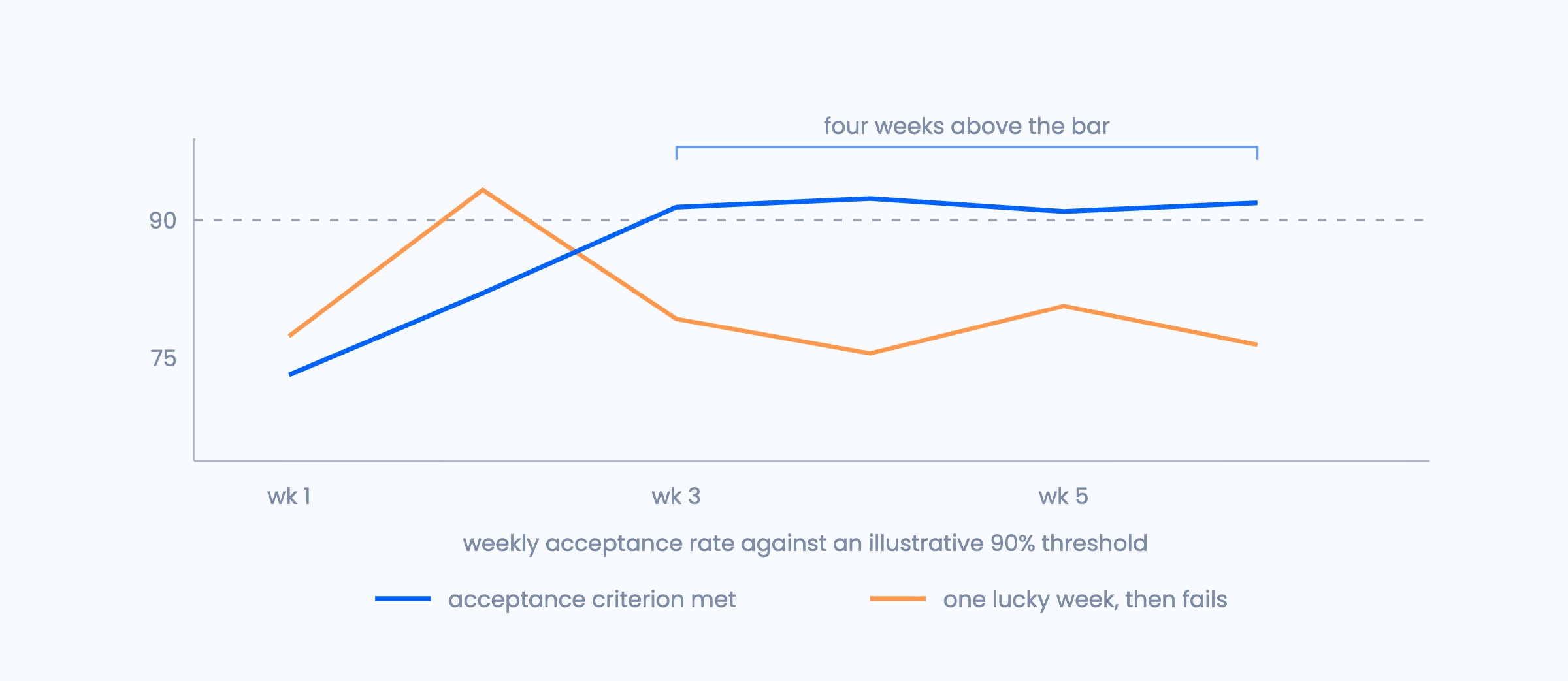
Optimizing for acceptance also creates a corruptible target, the problem associated with Goodhart's law: “When a measure becomes a target, it ceases to be a good measure.”^[12] Acceptance must be sustained rather than spiked, but four weeks alone do not prove quality. Accepted proposals need outcome checks; rejected proposals need decision-time reviews and outcome evidence where available. The grading of record is the decision quality acceptance is supposed to proxy, not acceptance itself.

Acceptance is necessary and not sufficient, because it measures the system against a person rather than against the operation. Review is the first stage where approved system calls execute, and promotion requires those orders to be non-inferior to the incumbent process on the merchant-defined outcomes, at minimum on-time performance and fully loaded cost, within margins agreed in advance.

For example:

If the allowed decline is 1.0 percentage point, the relevant lower confidence bound must clear −1.0, under the agreed statistical design. The positive observed difference alone does not establish non-inferiority.

Sample size decides whether it does. Under a simple independent two-sample illustration with 2,000 orders on each side:

The lower bound is 0.4 − 1.96 × 0.60 ≈ −0.79, above −1.0, so it passes. With 1,000 orders on each side, SE(Δ) ≈ 0.86 points and the lower bound is about −1.28. Same +0.4, but the smaller sample does not establish non-inferiority. The margin sets the tolerated decline; the confidence bound determines whether the evidence clears it.

The outcome comparison is reported separately from acceptance because its sample contains proposals reviewers chose to execute, not every proposal the system would have made. If dispatchers approve easy orders and intervene on difficult ones, the accepted sample has a selection advantage. Comparison within the same segment and period is a starting point; evaluation must address order mix and other differences, using stronger experimental designs where feasible.^[4][5]

A system that matches an adequate incumbent and is accepted by an accommodating reviewer passes the first two gates. It does not pass the outcome gate unless executed performance supports the agreed standard.

7. Grade judgment, not hindsight

A decision must be graded on what was knowable when it was made, against alternatives that were actually available. Outcome-only grading punishes good decisions that met bad luck and rewards bad decisions that got away with it, corrupting the record precisely where it matters most: the marginal cases.

A reasonable call meets a breakdown. On another installation order, the dispatcher approves B after checking crew availability, price, and window. The truck then breaks down, and the appointment is missed. That failure belongs in the outcome measures, but the breakdown does not automatically make the original choice unreasonable. Conversely, choosing A despite a known delay may work out because the building makes an exception; the lucky result does not erase the ignored risk.

The operational requirement is counterfactual preservation: keep the alternatives considered, their prices, and the constraint version in force, so a decision can be reassessed later without asking anyone to remember it. This preserves the decision-time comparison; it does not create an observed outcome for an unchosen alternative.

In Burq Intelligence, the Decision Ledger is that record of the call. The Decision Graph connects operating history: how providers have accepted, arrived, and held their prices by zone, hour, and order type. As the familiar modeling warning puts it, “All models are wrong, but some are useful.”^[13] The record makes usefulness something the operation can test and inspect.

The grader must also be independent of the decider it grades. Where the system's call did not execute, assessment can draw on the Decision Graph's observed record for that alternative on comparable orders, rather than the system's own forecast. A model that overrates a provider should not automatically overrate its decision to pick it.

That history remains an estimate for the road not taken, subject to selection and missing information. The grader is checked against orders with known outcomes, and where the alternative's record is too thin to support grading, the divergence stays ungraded and outside both the numerator and denominator of the productive-disagreement rate. Coverage and uncertainty remain visible beside the score.

8. The asymmetry: promotion offered, demotion automatic

The two authority transitions are deliberately unlike each other. Promotion is an evidence gate crossed, followed by a human signature: the system surfaces the evidence and waits. Demotion is a circuit breaker: a detected hard-rule breach, such as a dropoff outside dock hours, suspends the segment's authority automatically, with the evidence attached and no meeting required.

The asymmetry follows the different costs of error. Granting authority too early exposes subsequent orders to an unvalidated decider; the exposure grows with volume. Delaying authority keeps the current process in control while the team gathers evidence, although it may defer benefits. Make the expansion deliberate and human, and the protective withdrawal automatic.

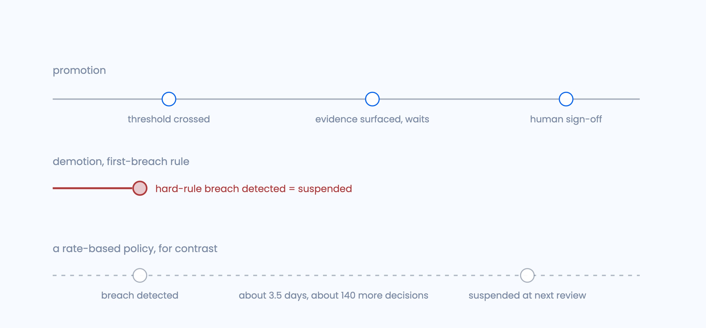
The dock closes before the truck arrives. Suppose the installation segment is now Autonomous and a delivery arrives after the hard 4 p.m. cutoff. Once detected, that breach suspends authority and routes subsequent work to the agreed fallback. The team does not wait for the weekly breach rate to worsen.

First-breach suspension is a policy choice for rules designated hard. Under an independent, constant per-decision breach probability q, the chance of reaching k decisions without a breach is:

The expected number of decisions through the first breach is:

At an illustrative q = 0.01, this is 100 decisions. That describes exposure under those assumptions, not a forecast for a real segment. A rate-based policy may leave the system deciding after a breach while it waits for enough evidence to trigger action. The lag is the exposure. And it can be counted. Assuming breaches are detected uniformly between weekly reviews, a segment making 40 decisions a day keeps deciding for about 3.5 days on average after a breach is detected, roughly 140 more decisions by a system that has already broken a hard rule. First-breach suspension takes that additional policy exposure to zero.

Revocation cannot prevent the first breach or shorten the time needed to detect one: a missed dock window may appear only at delivery or reconciliation. It removes the additional policy delay between detection and withdrawal, subject to execution latency. Where a hard rule is checkable before execution, validation should block the invalid call; revocation addresses breaches visible only afterward.

The operations team agrees in advance which events trigger withdrawal, who takes over, and how affected orders are handled. A circuit breaker needs a working handoff, not merely a status change.

9. Why the evidence must be live

Historical replay is seductive: run the model over last quarter's orders, compare against what the team did, and produce an agreement rate overnight. Replay can help prepare and diagnose a deployment. As evidence for granting authority, it leaves three important gaps.

The counterfactual is censored. Replay can say what the model would have chosen, but usually not what would have happened next. Whether the alternative provider would have accepted, arrived in the window, or changed its price is unobserved for that order. History contains outcomes for choices actually executed. This is a selection problem, not merely a data-volume problem, and more history does not automatically cure it.^[7]

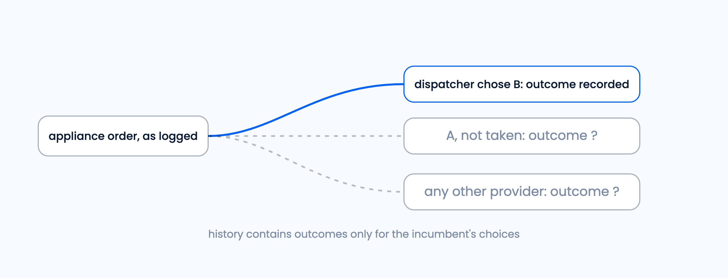
Decision-time information may be incomplete. Replaying the first appliance order might show A at $84 and B at $87 but omit A's delay call. Quotes expire, capacity changes, and constraint versions evolve. A reconstructed choice may therefore use only an approximation of what was knowable. Replay should report those limits rather than count an unavailable saving as a win.

The operation reacts. Dispatchers may work differently when proposals appear, and providers may respond to different order flow. A backtest cannot establish all those effects. The experimentation lesson is to evaluate the treatment in the world that will receive it.^[5]

Live Shadow improves the decision-time comparison, but only the dispatcher's call executes. It does not reveal the outcome of the system's alternative or establish how the full autonomous operation will behave. Review is the first stage where approved system calls produce outcomes of their own and the team can examine how recommendations change the workflow.

Replay may orient, but authority is earned only on live orders. In Shadow, the system's calls do not execute; what it costs is patience, plus integration and evaluation work the team should plan for.

10. The doctrine, instrumented: a worked example

The approach is implemented as Burq Intelligence, using the Decision Graph as operating context and the Decision Ledger as the record of each call. The following worked example shows the kind of board an operations team inspects for each segment. These are illustrative assumptions, not published deployment results or universal thresholds.

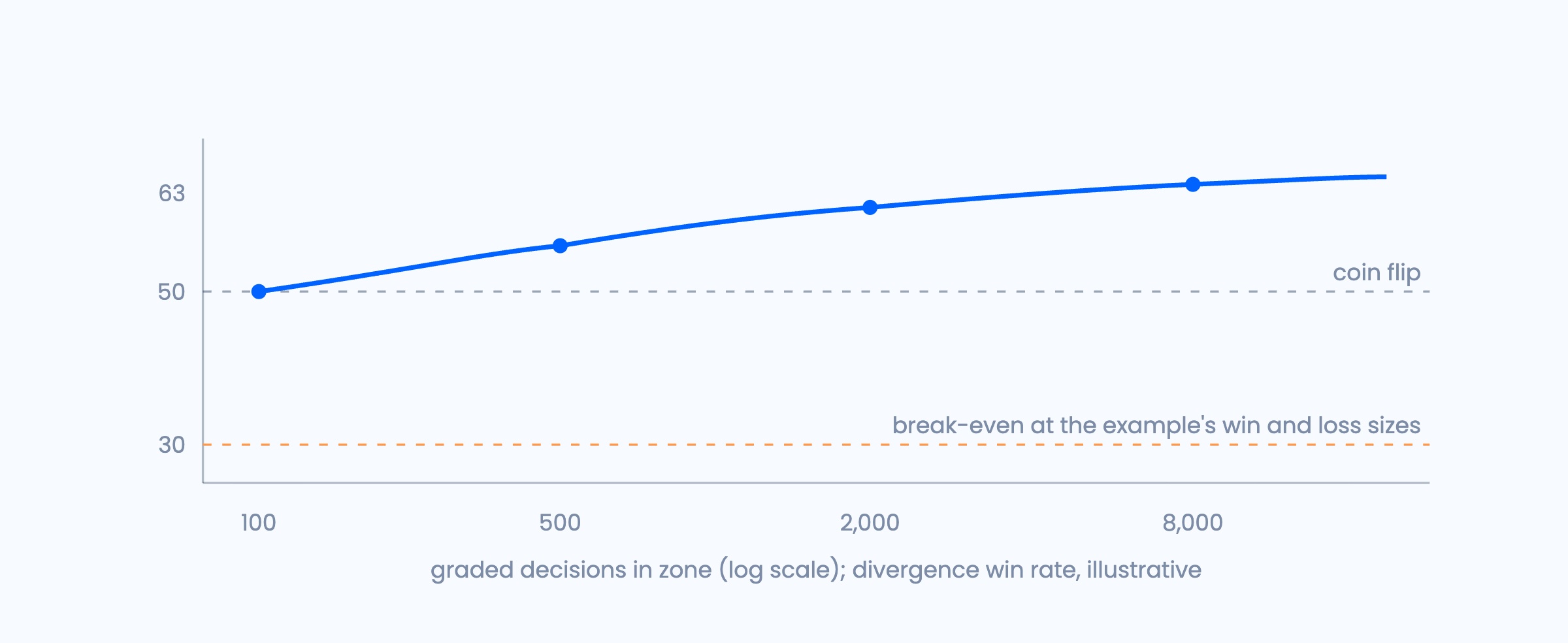
Two numbers carry the argument. The first is the productive-disagreement rate. On calls like the appliance orders, where the paths differ and can be assessed, the example favors the system 63% of the time. A win rate alone is not an economic result; wins and losses need pricing:

The size of wins and losses matters as much as the win rate. Setting value to zero gives the break-even win rate:

In this example, the system creates value as long as it wins more than three graded divergences in ten. The 63% carries its own uncertainty: with 200 graded divergences treated as independent, SE ≈ √(0.63 × 0.37 ÷ 200) ≈ 0.034, an interval of roughly 56% to 70%, comfortably above both a coin flip and break-even. The interval describes win-rate uncertainty; estimating uncertainty in dollar value also requires the distribution of savings and losses.

For an operation with 200,000 eligible orders a year:

The calculation assumes all divergences can be graded and the stated averages apply to them. With partial coverage, value is estimated only for the graded cases; the rest remains unknown unless additional evidence supports an estimate. If only 60% can be graded, the identified figure is 58,000 × 0.60 × $1.472 ≈ $51,000, and the remainder is unknown: not zero, and not another $34,000. This is potential value on paper, not realized savings. Executed outcomes, implementation costs, and service effects determine what the operation actually gains. The smaller losses than wins are assumptions in this example, not a guaranteed consequence of equivalence bands.

The other number is the demotion rate. A doctrine whose circuit breaker never trips should be suspected of not having one. The dock-hours incident shows what to inspect: the trigger, the suspension, the fallback, and the recovery. The breaker also has to be tested on purpose, because frequency alone doesn't prove it works.

Zero events don't prove a zero breach rate, either. After n clean decisions, a rough 95% upper bound on q is 3 ÷ n, the rule of three: 600 independent decisions with no observed breaches give an approximate 95% upper bound of 0.5%, not proof that q is zero. And at q = 0.1%, a segment running 1,000 decisions has a 1 − 0.999^1,000 ≈ 63% chance of at least one breach.

The economics have a structural hypothesis behind them. Dispatchers hold valuable local experience, including information like A's phone call. The Decision Graph complements that experience with a broader record across providers and operating conditions. Shadow adds paired human-versus-system choices; Review adds override reasons and executed outcomes. Together, they give the team material for learning and evaluation that immediate autonomous deployment does not automatically produce.

The prediction is that disagreements become more valuable where the record grows richer. That is the compounding-asset claim stated so it can fail. The team should test it against comparable work and control for changes in provider and order mix. If the curve is flat, the record is bookkeeping; if it rises under controlled comparisons, the record is the product.

11. What the doctrine refuses

Three deployment patterns are explicitly rejected.

Granted autonomy: full authority on integration day, evaluation deferred to the vendor's benchmark. Connecting an account establishes access, not readiness to act.

Benchmark theater: leaderboard performance offered as evidence about an operation the benchmark never saw. A benchmark may provide useful information, but it does not establish readiness for that merchant's constraints and delivery promises.

The permanent disclaimer: human-in-the-loop as a liability posture rather than a stage: review forever, thresholds never. It is a design that converts the most expensive resource in the building into a full-time rubber stamp and calls it safety. A team can legitimately keep high-risk work in Review, but the review should have a clear purpose rather than remain an unexamined default.

12. Open problems

Honest doctrine names its unfinished edges. The structure is settled: how authority is earned, what withdraws it, and what the record must hold. The settings inside it are calibrated from each operation's own record, segment by segment, and the methods for some of that calibration are still open.

Threshold calibration. Equivalence bands and promotion thresholds are risk decisions that belong to the merchant, but merchants deserve better guidance than folklore. A principled mapping from segment value-at-risk to (α, β, margins) remains open work. A low-cost routine delivery and a high-value installation should not automatically use the same risk settings.

Agreement under imbalance. κ behaves awkwardly when one provider dominates a segment, and the right chance-correction for priced, multi-alternative decisions is not settled. The diagnostic must be interpreted alongside feasible options, cost, and service commitments.

Weighting disagreement. The productive-disagreement rate is the escape from the incumbent ceiling, but how to weight it against raw agreement inside a promotion criterion, without rewarding disagreement for its own sake, remains a Goodhart problem. Two starting points are to credit checkable improvements, such as avoiding a policy breach or choosing an available option better on both price and window, and to measure how often dispatchers agree with each other. That human baseline provides context, not proof of outcome quality.

Drift. A threshold crossed once is not a threshold held forever. Once a segment is Autonomous, a dispatcher no longer decides beside it on every order, so the comparison signal shrinks just as continuing monitoring becomes critical. Suppose on-time performance slips a few tenths of a point each week. The approach tracks the promotion outcome measures against pre-specified rolling-window margins, with a sequential monitor designed to detect slow, persistent change rather than merely one bad day. Page's CUSUM is the classic version.^[14] Track the weekly late rate x against its promotion baseline μ₀, allow a slack k for ordinary noise, and accumulate only the excess:

The alarm fires when S crosses a threshold h. If the installation segment was promoted at a 4.0% late rate, with k = 0.25 points and h = 1.0 point, and its late rate slips to 4.3%, 4.6%, and 4.9% over three weeks, then S = 0.05, 0.40, and 1.05: no single week looks alarming, but the monitor fires in week three. These k and h values are illustrative; real settings need calibration to order volume, variability, and the false-alarm rate the team will accept. Crossing the agreed monitoring boundary returns the segment to Review, while a detected hard-rule breach suspends it immediately. A small sampled set of orders continues to receive parallel human calls so agreement and diagnostic evidence survive promotion. The cadence, dependence assumptions, and sensitivity of that monitor deserve the same advance specification as promotion.

Reviewer vigilance. Sustaining genuine review through months of mostly-right proposals is a human-factors problem no statistic fully solves.^[10][11] The Friday queue is a reminder that clear reasons, manageable workloads, and outcome checks matter alongside an acceptance rate.

These are the problems a record makes tractable. The record lets the team state them precisely, examine them, and check what changed after intervention. Earned autonomy turns trust into an operating process: define the work, set the bar, gather evidence, approve authority, and keep checking whether it remains justified.